Note
Go to the end to download the full example code.
Steady State Thermal Analysis of cooling holes on a representative model#
This example illustrates the process of adding a Steady State Thermal analysis to a new standalone Mechanical session, followed by executing Python scripting commands to set boundary conditions and solve a thermal simulation of a model with cooling holes. The scripts then assess the results, including temperature plots of plates and fluid lines modeled with Fluid116 elements.
Cooling holes are carefully designed small channels within turbine blades that release cool air, creating a protective layer on the blade’s surface to shield it from the intense heat of combustion gases. This film cooling technique helps maintain optimal temperatures, boost turbine efficiency, and ensure safe operation. The size, shape, and location of these holes are crucial for their effectiveness and to prevent premature failure.
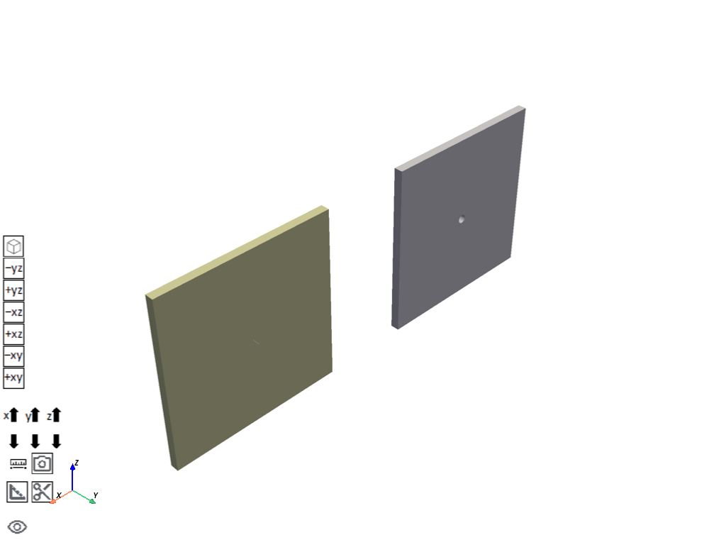
The model features two plates: one equipped with cooling holes and the other without them. Fluid116 elements simulate the flow network through the holes without requiring the holes to be physically present in the geometry.
The plates are constructed from structural steel, with air flowing through the holes. The simulation involves applying convection boundary conditions to the plate surfaces, temperature boundary conditions at the line vertices, and mass flow rate boundary conditions at the fluid lines. After solving the simulation, the results are visualized with temperature plots, showing the temperature distribution on the plates and fluid lines using matplotlib.
Import the necessary libraries#
from pathlib import Path
from typing import TYPE_CHECKING

from ansys.mechanical.core import App
from ansys.mechanical.core.examples import delete_downloads, download_file

if TYPE_CHECKING:
    import Ansys
Initialize the embedded application#
app = App(globals=globals())
print(app)

# Set the path for the output files (images, gifs, mechdat)
output_path = Path.cwd() / "out"
graphics = app.Graphics
camera = graphics.Camera
Ansys Mechanical [Ansys Mechanical Enterprise]
Product Version:261
Software build date: 01/30/2026 18:48:37
Download the required files#
# Download the geometry file
geometry_path = download_file("cooling_holes_geometry.pmdb", "pymechanical", "embedding")

# Download the material file
mat_path = download_file("cooling_holes_material_file.xml", "pymechanical", "embedding")
Define Python variables#
Store all main tree nodes as variables
model = app.Model
geometry = model.Geometry
mesh = model.Mesh
materials = model.Materials
coordinate_systems = model.CoordinateSystems
named_selections = model.NamedSelections
Import the geometry#
# Import the geometry with the specified settings
geometry_import = app.helpers.import_geometry(
    geometry_path,
    process_named_selections=True,
    process_coordinate_systems=True,
    named_selection_key="",
    process_material_properties=True,
)
Define and select BIN units system#
Define the unit system for the model as Standard BIN (BTU, inch).
app.ExtAPI.Application.ActiveUnitSystem = MechanicalUnitSystem.StandardBIN
Assign materials#
Import material from xml file and assign it to bodies
materials.Import(mat_path)
<System.Collections.Generic.List[Material] object at 0x7f150cbcfe00>
Assign geometrical and material properties#
Specify section properties and assign them to geometry
geometry.Activate()
fluid_line1 = geometry.Children[2].Children[0]  # Activate fluid line Body
fluid_line1.ModelType = PrototypeModelType.ModelPhysicsTypeFluid
fluid_line1.Material = "Air"
fluid_line1.FluidCrossArea = Quantity(3.1414, "in in")

fluid_line2 = geometry.Children[3].Children[0]  # Activate fluid line Body
fluid_line2.ModelType = PrototypeModelType.ModelPhysicsTypeFluid
fluid_line2.Material = "Air"
fluid_line2.FluidCrossArea = Quantity(3.1414, "in in")

# Visualize the model in 3D
app.plot()
[]
Define coordinate system#
Specify cylindrical coordinate system for applying boundary conditions
coordinate_systems.Activate()
coordinate_system_101 = coordinate_systems.AddCoordinateSystem()
coordinate_system_101.CoordinateSystemType = CoordinateSystemTypeEnum.Cylindrical
coordinate_system_101.OriginDefineBy = CoordinateSystemAlignmentType.Component
coordinate_system_101.OriginDefineBy = CoordinateSystemAlignmentType.Fixed
coordinate_system_101.OriginX = Quantity(2, "in")
coordinate_system_101.OriginZ = Quantity(-0.5, "in")
coordinate_system_101.PrimaryAxis = CoordinateSystemAxisType.PositiveZAxis
coordinate_system_101.PrimaryAxisDefineBy = CoordinateSystemAlignmentType.GlobalY
coordinate_system_101.SecondaryAxisDefineBy = CoordinateSystemAlignmentType.GlobalZ
Define named selections#
Create named selections used in the model
HoleFluidNodes_NS = [x for x in Tree.AllObjects if x.Name == "HoleFluidNodes"][0]
Both_Plates_NS = [x for x in Tree.AllObjects if x.Name == "Both_Plates"][0]
Fluid_Line1_NS = [x for x in Tree.AllObjects if x.Name == "Fluid_Line1"][0]
Fluid_Line2_NS = [x for x in Tree.AllObjects if x.Name == "Fluid_Line2"][0]
Line1_vertex_NS = [x for x in Tree.AllObjects if x.Name == "Line1_vertex"][0]
Line2_vertex_NS = [x for x in Tree.AllObjects if x.Name == "Line2_vertex"][0]
Bottom_Surface_Plates_NS = [x for x in Tree.AllObjects if x.Name == "Bottom_Surface_Plates"][0]
Top_Surface_Plates_NS = [x for x in Tree.AllObjects if x.Name == "Top_Surface_Plates"][0]
Hole_Cyl_Surface_NS = [x for x in Tree.AllObjects if x.Name == "Hole_Cyl_Surface"][0]
Fluidlines_NS = [x for x in Tree.AllObjects if x.Name == "Fluidlines"][0]

# Create named selection for elements at the hole
named_selections = model.NamedSelections
named_selection = named_selections.AddNamedSelection()
named_selection.ScopingMethod = GeometryDefineByType.Worksheet
named_selection.GenerationCriteria.Add(None)
named_selection.GenerationCriteria[0].EntityType = SelectionType.MeshElement
named_selection.GenerationCriteria[0].Criterion = SelectionCriterionType.LocationX
named_selection.GenerationCriteria[0].Operator = SelectionOperatorType.LessThanOrEqual
named_selection.GenerationCriteria[0].Value = Quantity("2.5e-2 [in]")
cyl_cs = DataModel.GetObjectsByName("Coordinate System")
named_selection.GenerationCriteria[0].CoordinateSystem = cyl_cs[0]
named_selection.GenerationCriteria.Add(None)
named_selection.GenerationCriteria[1].Action = SelectionActionType.Convert
named_selection.GenerationCriteria[1].EntityType = SelectionType.MeshNode
active_sel = named_selection.GenerationCriteria[1]
active_sel.Active = False
named_selection.Generate()
named_selection.Name = r"""HoleElements"""
Define mesh controls and generate the mesh#
Mesh the model
mesh.Activate()
mesh.ElementSize = Quantity(0.5, "in")
mesh.UseAdaptiveSizing = False
mesh.CaptureCurvature = True
mesh.CaptureProximity = True
mesh.GrowthRateSF = 1.85
mesh.DefeatureTolerance = Quantity(0.000375, "in")

automatic_method = mesh.AddAutomaticMethod()
automatic_method.ScopingMethod = GeometryDefineByType.Component
automatic_method.NamedSelection = Both_Plates_NS
automatic_method.Method = MethodType.AllTriAllTet

sizing = mesh.AddSizing()
sizing.ScopingMethod = GeometryDefineByType.Component
sizing.NamedSelection = Fluidlines_NS
sizing.ElementSize = Quantity(1e-2, "in")
sizing.CaptureCurvature = False
sizing.CaptureProximity = False
mesh.GenerateMesh()
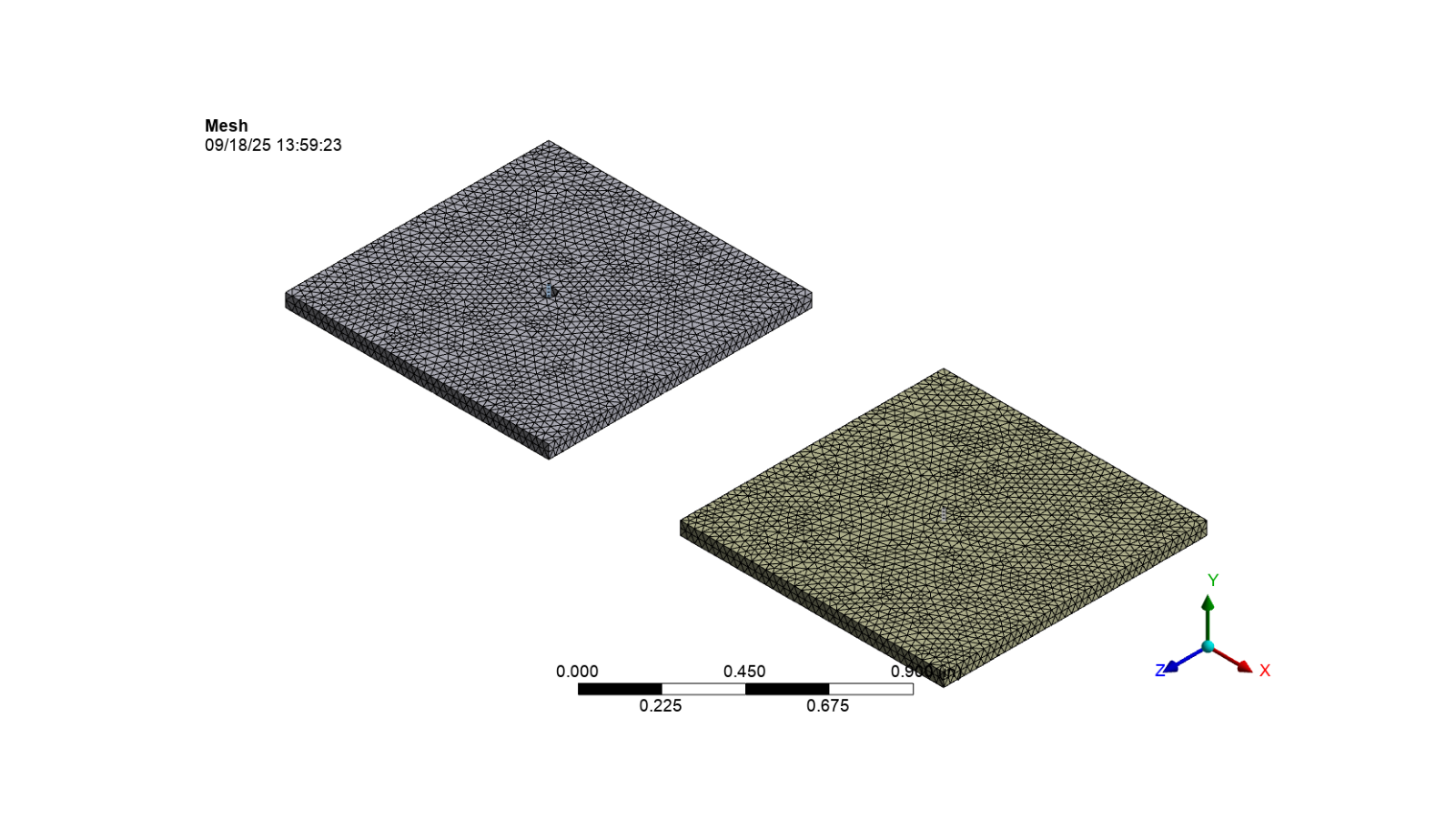
Display the mesh
# Activate the mesh for visualization
app.Tree.Activate([mesh])

# Set the camera to fit the model and export the image
camera.SetFit()
image_path = output_path / "mesh.png"
app.helpers.export_image(mesh, image_path)
app.helpers.display_image(image_path)
Define analysis#
Add a Steady State Thermal Analysis
steady_state_thermal = model.AddSteadyStateThermalAnalysis()
steady_state_thermal_analysis = model.Analyses[0].AnalysisSettings

# Define the static structural analysis solution
solution = model.Analyses[0].Solution
/__w/pymechanical/pymechanical/examples/01_basic/cooling_holes_thermal_analysis.py:249: UserWarning: Obsolete: 'AnalysisSettings': Property is obsolete, use IAnalysisSettings instead.
  steady_state_thermal_analysis = model.Analyses[0].AnalysisSettings
Apply loads and boundary conditions#
Add convection loads, body temperatures, and mass flow rates
steady_state_thermal.Activate()

# Apply convection at the surfaces
convection_1 = steady_state_thermal.AddConvection()
convection_1.Location = Top_Surface_Plates_NS
convection_1.FilmCoefficient = Quantity(2.9e-4, "BTU sec^-1 in^-1 in^-1 F^-1")
convection_1.AmbientTemperature = Quantity(1700, "F")

convection_2 = steady_state_thermal.AddConvection()
convection_2.Location = Bottom_Surface_Plates_NS
convection_2.FilmCoefficient = Quantity(5e-4, "BTU sec^-1 in^-1 in^-1 F^-1")
convection_2.AmbientTemperature = Quantity(900, "F")

convection_3 = steady_state_thermal.AddConvection()
convection_3.Location = Hole_Cyl_Surface_NS
convection_3.FilmCoefficient = Quantity(9.65e-4, "BTU sec^-1 in^-1 in^-1 F^-1")
convection_3.AmbientTemperature = Quantity(900, "F")
convection_3.HasFluidFlow = True
convection_3.DisplayConnectionLines = True
convection_3.FluidFlowSelection = Fluid_Line1_NS

# Apply temperature at the line vertices
temperature_1 = steady_state_thermal.AddTemperature()
temperature_1.Location = Line1_vertex_NS
temperature_1.Magnitude = Quantity(900, "F")

temperature_2 = steady_state_thermal.AddTemperature()
temperature_2.Location = Line2_vertex_NS
temperature_2.Magnitude = Quantity(900, "F")

# Apply mass flow rate at the fluid lines
mass_flow_rate_1 = steady_state_thermal.AddMassFlowRate()
mass_flow_rate_1.Location = Fluid_Line1_NS
mass_flow_rate_1.Magnitude.Output.SetDiscreteValue(0, Quantity(9.9999e-4, "lbm sec^-1"))

mass_flow_rate_2 = steady_state_thermal.AddMassFlowRate()
mass_flow_rate_2.Location = Fluid_Line2_NS
mass_flow_rate_2.Magnitude.Output.SetDiscreteValue(0, Quantity(9.9999e-4, "lbm sec^-1"))
Insert command snippet to create surface effect elements at the hole#
command_snippet = steady_state_thermal.AddCommandSnippet()

command_snippet.Input = r"""

FINISH

/prep7
cmsel,s,HoleElements        !Select elements that represent where the hole is
nsle,s                                      !Select the nodes for these elements
cm,holenodes,node           !Store the nodes for these elements as a component

esel,inve                       !Switch selection to inverse of these elements
esel,r,ename,,291       !Reselect just the solid elements
nsle,s                                  !Select the nodes for these elements
cmsel,r,holenodes       !reselect nodes from the holenodes component
                        !results in nodes at the interfaces being selected

/com, now nodes at the interface are selected and elements
/com, (minus the elements where the hole would be) are selected
/com, Create a new surface effect element type

*get,maxetyp,ETYP,0,NUM,MAX
newsurftyp=maxetyp+1
ET,newsurftyp,SURF152
mat,newsurftyp
type,newsurftyp
real,newsurftyp
esurf,all

KEYOPT,newsurftyp,5,1
KEYOPT,newsurftyp,8,2

/com, Now need to attach these new surface effect elements to the fluid 116 elements
/com, that pass through where the hole will be store the element centroids of the new
/com, surface effect elements using mask arrays. First get a list of the new surface
/com, effect elements and the mask array
esel,s,type,,newsurftyp
*del,elemnums,,nopr
*vget,elemnums,elem,,elist
*del,elemmask,,nopr
*vget,elemmask,elem,,esel

/com, Get count of new surface effect elements and maxelement number for loops
*get,surfelemcount,elem,,count
*get,maxelem,elem,,num,maxd

/com, store array of all centroids in model
*del,elemcent,,nopr
*dim,elemcent,array,maxelem,3
*vget,elemcent(1,1),elem,,cent,x
*vget,elemcent(1,2),elem,,cent,y
*vget,elemcent(1,3),elem,,cent,z

/com, Compress down to centroids of new surface effect elements
*del,surfelemcent,,nopr
*dim,surfelemcent,array,surfelemcount,3
*vmask,elemmask
*vfun,surfelemcent(1,1),comp,elemcent(1,1)
*vmask,elemmask
*vfun,surfelemcent(1,2),comp,elemcent(1,2)
*vmask,elemmask
*vfun,surfelemcent(1,3),comp,elemcent(1,3)
*del,elemcent,,nopr
*del,elemmask,,nopr

cmsel,s,holefluidnodes

/com, Loop through each surface effect element and find the closest fluid node
/com, then assign it as the extra node for that surface effect element
totalarea=0
*do,eliter,1,surfelemcount,1
    closestnode=node(surfelemcent(eliter,1),surfelemcent(eliter,2),surfelemcent(eliter,3))
    !For SURF152 elements with midside nodes (KEYOPT4=0)
    emodif,elemnums(eliter),-9,closestnode
    *get,elemarea,elem,elemnums(eliter),area
    totalarea=totalarea+elemarea
*enddo

/com, Add convection boundary conditions to new surface effect elements.
/com, Use expected hole surface area ratioed to actual surface effect element area
/com, to dial in proper heat transfer
/solu
alls
esel,s,type,,newsurftyp
ApplyHTC = 9.65e-4*778.2*12         !Convert to proper units, in BIN so convert BTU to in-lbf

/com, Calculate expected hole area (here it is calculated as a straight hole with known
/com, diameter and length). Could also just hardcode in surface area of the hole
HoleDia = 0.05
HoleLength = 0.05
HoleArea = 3.141592654*HoleDia*HoleLength

/com, Adjust HTC by ratio of desired area vs actual surface effect area
AdjustHTC = ApplyHTC*HoleArea/totalarea
sf,all,conv,AdjustHTC,900

alls """
Insert results#
Insert temperature results
temp_plot_both_plates = solution.AddTemperature()
temp_plot_both_plates.Location = Both_Plates_NS
temp_plot_fluidlines = solution.AddTemperature()
temp_plot_fluidlines.Location = Fluidlines_NS
Solve#
solution.Solve(True)
STAT_SS = solution.Status
Postprocessing#
camera.SetFit()
camera.SceneHeight = Quantity(2.0, "in")
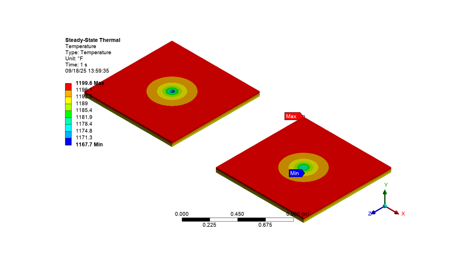
Display the temperature plots for both plates
# Activate the temperature results for both plates
app.Tree.Activate([temp_plot_both_plates])
# Set the extra model display to no wireframe
app.Graphics.ViewOptions.ResultPreference.ExtraModelDisplay = (
    Ansys.Mechanical.DataModel.MechanicalEnums.Graphics.ExtraModelDisplay.NoWireframe
)
# Set the camera to fit the model and export the image
image_path = output_path / "temp_plot_both_plates.png"
app.helpers.export_image(temp_plot_both_plates, image_path)
# Display the exported image
app.helpers.display_image(image_path)
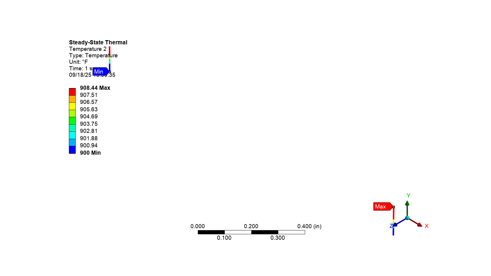
Display the temperature plots for fluid lines
# Activate the temperature results for fluid lines
app.Tree.Activate([temp_plot_fluidlines])
# Set the camera to fit the model and export the image
image_path = output_path / "temp_plot_fluidlines.png"
app.helpers.export_image(temp_plot_fluidlines, image_path)
# Display the exported image
app.helpers.display_image(image_path)
Clean up the project#
# Save the project
mechdat_file = output_path / "cooling_holes_model.mechdat"
app.save_as(str(mechdat_file), overwrite=True)

# Close the app
app.close()

# Delete the example file
delete_downloads()
True
Total running time of the script: (0 minutes 28.708 seconds)