Note
Go to the end to download the full example code.
Steady state thermal analysis#
This example problem demonstrates the use of a simple steady-state thermal analysis to determine the temperatures, thermal gradients, heat flow rates, and heat fluxes that are caused by thermal loads that do not vary over time. A steady-state thermal analysis calculates the effects of steady thermal loads on a system or component, in this example, a long bar model.
Import the necessary libraries#
from pathlib import Path
from typing import TYPE_CHECKING

from matplotlib import pyplot as plt
from matplotlib.animation import FuncAnimation
from PIL import Image

from ansys.mechanical.core import App
from ansys.mechanical.core.examples import delete_downloads, download_file

if TYPE_CHECKING:
    import Ansys
Initialize the embedded application#
app = App(globals=globals())
print(app)

# Set the path for the output files (images, gifs, mechdat)
output_path = Path.cwd() / "out"

# Set the camera orientation to isometric view
graphics = app.Graphics
camera = graphics.Camera

# Set the camera orientation to isometric view
camera.SetSpecificViewOrientation(ViewOrientationType.Iso)
Ansys Mechanical [Ansys Mechanical Enterprise]
Product Version:261
Software build date: 01/30/2026 18:48:37
Download the geometry file#
# Download the geometry file from the ansys/example-data repository
geometry_path = download_file("LONGBAR.x_t", "pymechanical", "embedding")
Import the geometry#
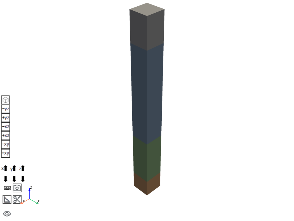
app.helpers.import_geometry(geometry_path, process_named_selections=True)

# Visualize the model in 3D
app.plot()
[]
Add steady state thermal analysis#
# Add a steady state thermal analysis to the model
model = app.Model
model.AddSteadyStateThermalAnalysis()
# Set the Mechanical unit system to Standard MKS
app.ExtAPI.Application.ActiveUnitSystem = MechanicalUnitSystem.StandardMKS

# Get the steady state thermal analysis
stat_therm = model.Analyses[0]

# Add a coordinate system to the model
coordinate_systems = model.CoordinateSystems

# Add two coordinate systems
lcs1 = coordinate_systems.AddCoordinateSystem()
lcs1.OriginX = Quantity("0 [m]")

lcs2 = coordinate_systems.AddCoordinateSystem()
lcs2.OriginX = Quantity("0 [m]")
lcs2.PrimaryAxisDefineBy = CoordinateSystemAlignmentType.GlobalY
Create named selections and construction geometry#
Create a function to add a named selection
def setup_named_selection(name, scoping_method=GeometryDefineByType.Worksheet):
    """Create a named selection with the specified scoping method and name.

    Parameters
    ----------
    name : str
        The name of the named selection.
    scoping_method : GeometryDefineByType
        The scoping method for the named selection.

    Returns
    -------
    Ansys.ACT.Automation.Mechanical.NamedSelection
        The created named selection.
    """
    ns = model.AddNamedSelection()
    ns.ScopingMethod = scoping_method
    ns.Name = name
    return ns
Create a function to add generation criteria to the named selection
def add_generation_criteria(
    named_selection,
    value,
    set_active_action_criteria=True,
    active=True,
    action=SelectionActionType.Add,
    entity_type=SelectionType.GeoFace,
    criterion=SelectionCriterionType.Size,
    operator=SelectionOperatorType.Equal,
):
    """Add generation criteria to the named selection.

    Parameters
    ----------
    named_selection : Ansys.ACT.Automation.Mechanical.NamedSelection
        The named selection to which the criteria will be added.
    value : Quantity
        The value for the criteria.
    active : bool
        Whether the criteria is active.
    action : SelectionActionType
        The action type for the criteria.
    entity_type : SelectionType
        The entity type for the criteria.
    criterion : SelectionCriterionType
        The criterion type for the criteria.
    operator : SelectionOperatorType
        The operator for the criteria.
    """
    generation_criteria = named_selection.GenerationCriteria
    criteria = Ansys.ACT.Automation.Mechanical.NamedSelectionCriterion()

    set_criteria_properties(
        criteria,
        value,
        set_active_action_criteria,
        active,
        action,
        entity_type,
        criterion,
        operator,
    )

    if set_active_action_criteria:
        generation_criteria.Add(criteria)
Create a function to set the properties of the generation criteria
def set_criteria_properties(
    criteria,
    value,
    set_active_action_criteria=True,
    active=True,
    action=SelectionActionType.Add,
    entity_type=SelectionType.GeoFace,
    criterion=SelectionCriterionType.Size,
    operator=SelectionOperatorType.Equal,
):
    """Set the properties of the generation criteria.

    Parameters
    ----------
    criteria : Ansys.ACT.Automation.Mechanical.NamedSelectionCriterion
        The generation criteria to set properties for.
    active : bool
        Whether the criteria is active.
    action : SelectionActionType
        The action type for the criteria.
    entity_type : SelectionType
        The entity type for the criteria.
    criterion : SelectionCriterionType
        The criterion type for the criteria.
    operator : SelectionOperatorType
        The operator for the criteria.
    """
    if set_active_action_criteria:
        criteria.Active = active
        criteria.Action = action

    criteria.EntityType = entity_type
    criteria.Criterion = criterion
    criteria.Operator = operator
    criteria.Value = value

    return criteria
Add named selections to the model
face1 = setup_named_selection("Face1")
add_generation_criteria(face1, Quantity("20 [m]"), criterion=SelectionCriterionType.LocationZ)
face1.Activate()
face1.Generate()

face2 = setup_named_selection("Face2")
add_generation_criteria(face2, Quantity("0 [m]"), criterion=SelectionCriterionType.LocationZ)
face2.Activate()
face2.Generate()

face3 = setup_named_selection("Face3")
add_generation_criteria(face3, Quantity("1 [m]"), criterion=SelectionCriterionType.LocationX)
add_generation_criteria(
    face3,
    Quantity("2 [m]"),
    criterion=SelectionCriterionType.LocationY,
    action=SelectionActionType.Filter,
)
add_generation_criteria(
    face3,
    Quantity("12 [m]"),
    criterion=SelectionCriterionType.LocationZ,
    action=SelectionActionType.Filter,
)
add_generation_criteria(face3, Quantity("4.5 [m]"), criterion=SelectionCriterionType.LocationZ)
add_generation_criteria(
    face3,
    Quantity("2 [m]"),
    criterion=SelectionCriterionType.LocationY,
    action=SelectionActionType.Filter,
)
face3.Activate()
face3.Generate()

body1 = setup_named_selection("Body1")
body1.GenerationCriteria.Add(None)
set_criteria_properties(
    body1.GenerationCriteria[0],
    Quantity("1 [m]"),
    set_active_action_criteria=False,
    criterion=SelectionCriterionType.LocationZ,
)
body1.GenerationCriteria.Add(None)
set_criteria_properties(
    body1.GenerationCriteria[1],
    Quantity("1 [m]"),
    set_active_action_criteria=False,
    criterion=SelectionCriterionType.LocationZ,
)
body1.Generate()
Create construction geometry
# Add construction geometry to the model
construction_geometry = model.AddConstructionGeometry()
# Add a path to the construction geometry
construction_geom_path = construction_geometry.AddPath()

# Set the coordinate system for the construction geometry path
construction_geom_path.StartYCoordinate = Quantity(2, "m")
construction_geom_path.StartZCoordinate = Quantity(20, "m")
construction_geom_path.StartZCoordinate = Quantity(20, "m")
construction_geom_path.EndXCoordinate = Quantity(2, "m")

# Add a surface to the construction geometry
surface = construction_geometry.AddSurface()
# Set the coordinate system for the surface
surface.CoordinateSystem = lcs2
# Update the solids in the construction geometry
construction_geometry.UpdateAllSolids()
Define the boundary condition and add results#
Create a function to set the location and output for the temperature boundary condition
def set_loc_and_output(temp, location, values):
    """Add a temperature set output to the boundary condition.

    Parameters
    ----------
    temp : Ansys.Mechanical.DataModel.SteadyStateThermal.Temperature
        The temperature boundary condition.
    location : Ansys.Mechanical.DataModel.Geometry.GeometryObject
        The location of the temperature boundary condition.
    values : list[Quantity]
        The list of values for the temperature.
    """
    temp.Location = location
    temp.Magnitude.Output.DiscreteValues = [Quantity(value) for value in values]
Create a function to set the inputs and outputs for the temperature boundary condition
def set_inputs_and_outputs(
    condition,
    input_quantities: list = ["0 [sec]", "1 [sec]", "2 [sec]"],
    output_quantities: list = ["22[C]", "30[C]", "40[C]"],
):
    """Set the temperature inputs for the boundary condition.

    Parameters
    ----------
    condition : Ansys.Mechanical.DataModel.SteadyStateThermal.Temperature
        The temperature boundary condition.
    inputs : list[Quantity]
        The list of input values for the temperature.
    """
    # Set the magnitude for temperature or the ambient temperature for radiation
    if "Temperature" in str(type(condition)):
        prop = condition.Magnitude
    elif "Radiation" in str(type(condition)):
        prop = condition.AmbientTemperature

    # Set the inputs and outputs for the temperature or radiation
    prop.Inputs[0].DiscreteValues = [Quantity(value) for value in input_quantities]
    prop.Output.DiscreteValues = [Quantity(value) for value in output_quantities]
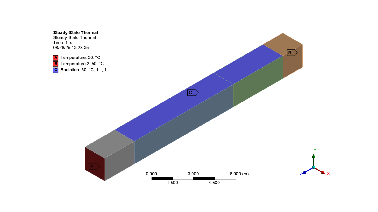
Add temperature boundary conditions to the steady state thermal analysis
temp = stat_therm.AddTemperature()
set_loc_and_output(temp, face1, ["22[C]", "30[C]"])
temp2 = stat_therm.AddTemperature()
set_loc_and_output(temp2, face2, ["22[C]", "60[C]"])

set_inputs_and_outputs(temp)
set_inputs_and_outputs(temp2, output_quantities=["22[C]", "50[C]", "80[C]"])
Add radiation
# Add a radiation boundary condition to the steady state thermal analysis
radiation = stat_therm.AddRadiation()
radiation.Location = face3
set_inputs_and_outputs(radiation)
radiation.Correlation = RadiationType.SurfaceToSurface
Set up the analysis settings
analysis_settings = stat_therm.AnalysisSettings
analysis_settings.NumberOfSteps = 2
analysis_settings.CalculateVolumeEnergy = True

# Activate the static thermal analysis and display the image
image_path = output_path / "bc_steady_state.png"
camera.SetFit()
app.helpers.export_image(stat_therm, image_path)
app.helpers.display_image(image_path)
/__w/pymechanical/pymechanical/examples/01_basic/steady_state_thermal_analysis.py:384: UserWarning: Obsolete: 'AnalysisSettings': Property is obsolete, use IAnalysisSettings instead.
  analysis_settings = stat_therm.AnalysisSettings
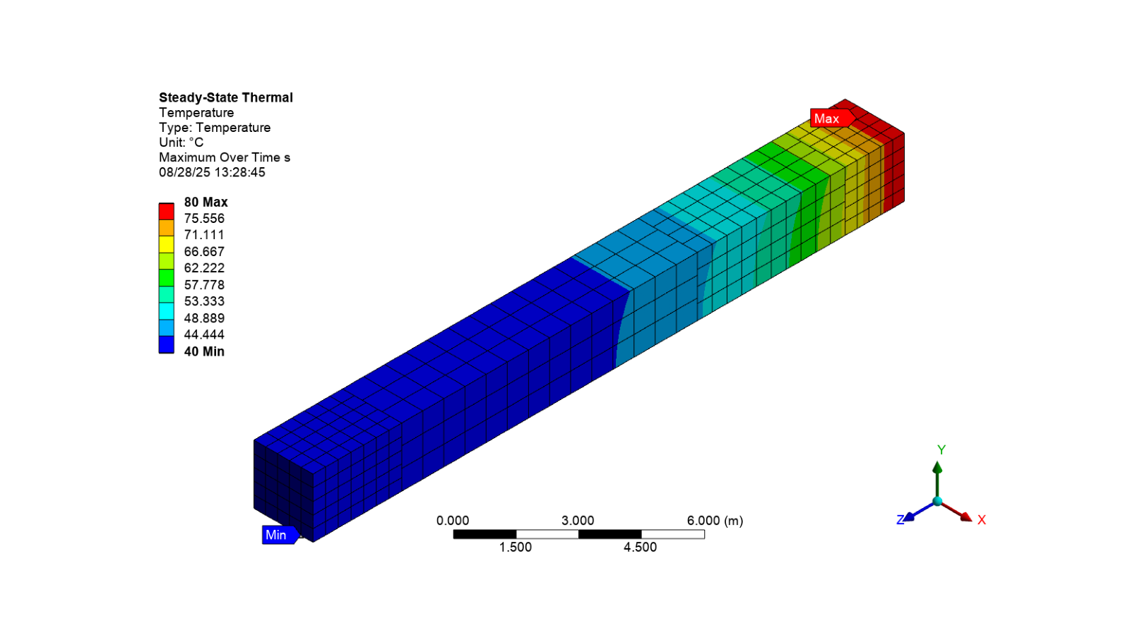
Add results#
Add temperature results to the solution
# Get the solution object for the steady state thermal analysis
stat_therm_soln = model.Analyses[0].Solution

# Add four temperature results to the solution
temp_rst = stat_therm_soln.AddTemperature()
temp_rst.By = SetDriverStyle.MaximumOverTime

# Set the temperature location to the body1 named selection
temp_rst2 = stat_therm_soln.AddTemperature()
temp_rst2.Location = body1

# Set the temperature location to the construction geometry path
temp_rst3 = stat_therm_soln.AddTemperature()
temp_rst3.Location = construction_geom_path

# Set the temperaature location to the construction geometry surface
temp_rst4 = stat_therm_soln.AddTemperature()
temp_rst4.Location = surface
Add the total and directional heat flux to the solution
total_heat_flux = stat_therm_soln.AddTotalHeatFlux()
directional_heat_flux = stat_therm_soln.AddTotalHeatFlux()

# Set the thermal result type and normal orientation for the directional heat flux
directional_heat_flux.ThermalResultType = TotalOrDirectional.Directional
directional_heat_flux.NormalOrientation = NormalOrientationType.ZAxis

# Set the coordinate system's primary axis for the directional heat flux
lcs2.PrimaryAxisDefineBy = CoordinateSystemAlignmentType.GlobalZ
directional_heat_flux.CoordinateSystem = lcs2

# Set the display option for the directional heat flux
directional_heat_flux.DisplayOption = ResultAveragingType.Averaged
Add thermal error and temperature probes
# Add a thermal error to the solution
thermal_error = stat_therm_soln.AddThermalError()

# Add a temperature probe to the solution
temp_probe = stat_therm_soln.AddTemperatureProbe()

# Set the temperature probe location to the face1 named selection
temp_probe.GeometryLocation = face1

# Set the temperature probe location method to the coordinate system
temp_probe.LocationMethod = LocationDefinitionMethod.CoordinateSystem
temp_probe.CoordinateSystemSelection = lcs2
Add a heat flux probe
hflux_probe = stat_therm_soln.AddHeatFluxProbe()

# Set the location method for the heat flux probe
hflux_probe.LocationMethod = LocationDefinitionMethod.CoordinateSystem
# Set the coordinate system for the heat flux probe
hflux_probe.CoordinateSystemSelection = lcs2
# Set the result selection to the z-axis for the heat flux probe
hflux_probe.ResultSelection = ProbeDisplayFilter.ZAxis
Add a reaction probe
# Update the analysis settings to allow output control nodal forces
analysis_settings.NodalForces = OutputControlsNodalForcesType.Yes

# Add a reaction probe to the solution
reaction_probe = stat_therm_soln.AddReactionProbe()
# Set the reaction probe geometry location to the face1 named selection
reaction_probe.LocationMethod = LocationDefinitionMethod.GeometrySelection
reaction_probe.GeometryLocation = face1
Add a radiation probe
radiation_probe = stat_therm_soln.AddRadiationProbe()
# Set the radiation probe boundary condition to the radiation boundary condition
radiation_probe.BoundaryConditionSelection = radiation
# Display all results for the radiation probe
radiation_probe.ResultSelection = ProbeDisplayFilter.All
Solve the solution#
# Solve the steady state thermal analysis solution
stat_therm_soln.Solve(True)
Show messages#
# Print all messages from Mechanical
app.messages.show()
Severity: Warning
DisplayString: A result is scoped to a construction geometry object which might have points shared with multiple bodies. Please check the results.   Object=Surface   Result=Temperature 4
Severity: Info
DisplayString: The requested license was received from the License Manager after 32 seconds.
Display the results#
# Activate the total body temperature and display the image
image_path = output_path / "total_body_temp.png"
camera.SetFit()
app.helpers.export_image(stat_therm, image_path)
app.helpers.display_image(image_path)
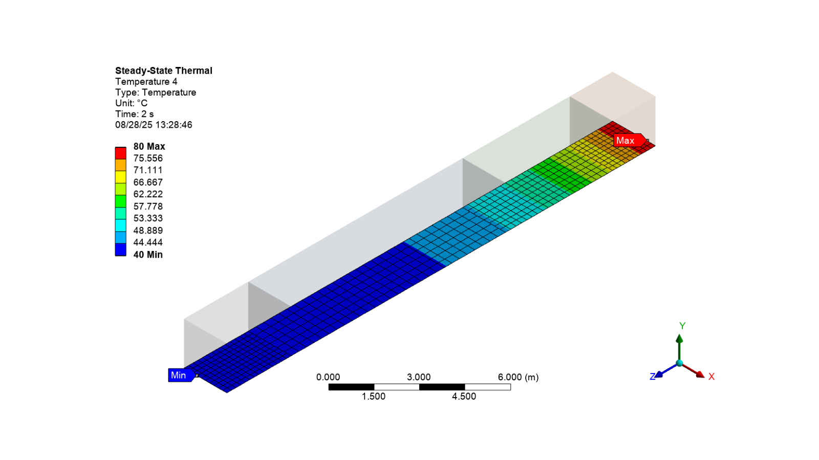
Temperature on part of the body
# Activate the temperature on part of the body and display the image
image_path = output_path / "part_temp_body.png"
camera.SetFit()
app.helpers.export_image(stat_therm, image_path)
app.helpers.display_image(image_path)
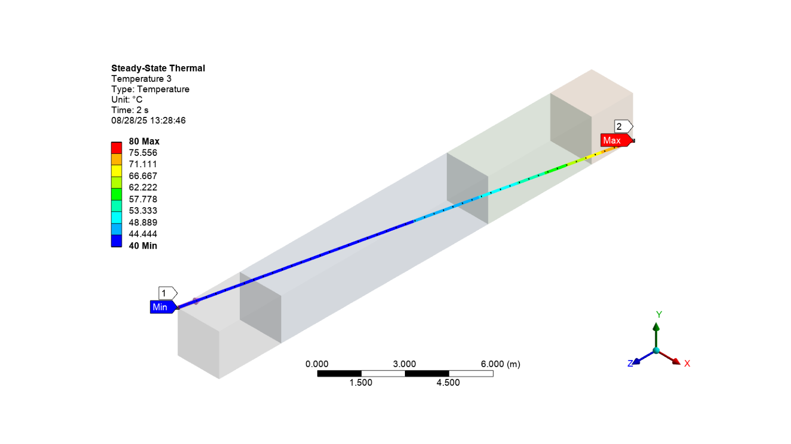
Temperature distribution along the specific path
# Activate the temperature distribution along the specific path and display the image
image_path = output_path / "path_temp_distribution.png"
camera.SetFit()
app.helpers.export_image(stat_therm, image_path)
app.helpers.display_image(image_path)
Temperature of bottom surface
# Activate the temperature of the bottom surface and display the image
image_path = output_path / "bottom_surface_temp.png"
camera.SetFit()
app.helpers.export_image(stat_therm, image_path)
app.helpers.display_image(image_path)
Export the directional heat flux animation#
# Export the directional heat flux animation as a GIF
directional_heat_flux_gif = output_path / "directional_heat_flux.gif"
app.helpers.export_animation(directional_heat_flux, directional_heat_flux_gif)
Display the heat flux animation#
# Open the GIF file and create an animation
gif = Image.open(directional_heat_flux_gif)
fig, ax = plt.subplots(figsize=(8, 4))
ax.axis("off")
image = ax.imshow(gif.convert("RGBA"))


# Animation update function
def update_frame(frame):
    """Update the frame for the animation."""
    gif.seek(frame)
    image.set_array(gif.convert("RGBA"))
    return (image,)


# Create and display animation
ani = FuncAnimation(fig, update_frame, frames=gif.n_frames, interval=200, blit=True, repeat=True)

# Show the animation
plt.show()
Display the output file from the solve#
# Get the working directory for the steady state thermal analysis
solve_path = Path(stat_therm.WorkingDir)
# Get the path to the solve.out file
solve_out_path = solve_path / "solve.out"
# Print the output of the solve.out file if applicable
if solve_out_path:
    with solve_out_path.open("rt") as file:
        for line in file:
            print(line, end="")
Ansys Mechanical Enterprise
*------------------------------------------------------------------*
| |
| W E L C O M E T O T H E A N S Y S (R) P R O G R A M |
| |
*------------------------------------------------------------------*
***************************************************************
* ANSYS MAPDL 2026 R1 LEGAL NOTICES *
***************************************************************
* *
* Copyright (c) 2026 Synopsys, Inc. and ANSYS, Inc. *
* All rights reserved. *
* Unauthorized use, distribution or duplication is *
* prohibited. *
* *
* Ansys is a registered trademark of Ansys, Inc. or its *
* subsidiaries in the United States or other countries. *
* See the Ansys, Inc. online documentation or the Ansys, Inc. *
* documentation CD or online help for the complete Legal *
* Notice. *
* *
***************************************************************
* *
* THIS ANSYS SOFTWARE PRODUCT AND PROGRAM DOCUMENTATION *
* INCLUDE TRADE SECRETS AND CONFIDENTIAL AND PROPRIETARY *
* PRODUCTS OF ANSYS, INC., ITS SUBSIDIARIES, OR LICENSORS. *
* The software products and documentation are furnished by *
* Ansys, Inc. or its subsidiaries under a software license *
* agreement that contains provisions concerning *
* non-disclosure, copying, length and nature of use, *
* compliance with exporting laws, warranties, disclaimers, *
* limitations of liability, and remedies, and other *
* provisions. The software products and documentation may be *
* used, disclosed, transferred, or copied only in accordance *
* with the terms and conditions of that software license *
* agreement. *
* *
* Ansys, Inc. is a UL registered *
* ISO 9001:2015 company. *
* *
***************************************************************
* *
* This product is subject to U.S. laws governing export and *
* re-export. *
* *
* For U.S. Government users, except as specifically granted *
* by the Ansys, Inc. software license agreement, the use, *
* duplication, or disclosure by the United States Government *
* is subject to restrictions stated in the Ansys, Inc. *
* software license agreement and FAR 12.212 (for non-DOD *
* licenses). *
* *
***************************************************************
2026 R1
Point Releases and Patches installed:
Ansys, Inc. License Manager 2026 R1
LS-DYNA 2026 R1
Core WB Files 2026 R1
Mechanical Products 2026 R1
***** MAPDL COMMAND LINE ARGUMENTS *****
BATCH MODE REQUESTED (-b) = NOLIST
INPUT FILE COPY MODE (-c) = COPY
DISTRIBUTED MEMORY PARALLEL REQUESTED
4 PARALLEL PROCESSES REQUESTED WITH SINGLE THREAD PER PROCESS
TOTAL OF 4 CORES REQUESTED
INPUT FILE NAME = /github/home/.mw/Application Data/Ansys/v261/AnsysMech9182/Project_Mech_Files/SteadyStateThermal/dummy.dat
OUTPUT FILE NAME = /github/home/.mw/Application Data/Ansys/v261/AnsysMech9182/Project_Mech_Files/SteadyStateThermal/solve.out
START-UP FILE MODE = NOREAD
STOP FILE MODE = NOREAD
RELEASE= 2026 R1 BUILD= 26.1 UP20260202 VERSION=LINUX x64
CURRENT JOBNAME=file0 20:08:28 JUL 13, 2026 Elapsed Time= 0.242
PARAMETER _DS_PROGRESS = 999.0000000
/INPUT FILE= ds.dat LINE= 0
*** NOTE *** ELAPSED TIME = 0.672 TIME= 20:08:28
The /CONFIG,NOELDB command is not valid in a distributed memory
parallel solution. Command is ignored.
*GET _WALLSTRT FROM ACTI ITEM=TIME WALL VALUE= 0.187360137E-03
TITLE=
--Steady-State Thermal
SET PARAMETER DIMENSIONS ON _WB_PROJECTSCRATCH_DIR
TYPE=STRI DIMENSIONS= 248 1 1
PARAMETER _WB_PROJECTSCRATCH_DIR(1) = /github/home/.mw/Application Data/Ansys/v261/AnsysMech9182/Project_Mech_Files/SteadyStateThermal/
SET PARAMETER DIMENSIONS ON _WB_SOLVERFILES_DIR
TYPE=STRI DIMENSIONS= 248 1 1
PARAMETER _WB_SOLVERFILES_DIR(1) = /github/home/.mw/Application Data/Ansys/v261/AnsysMech9182/Project_Mech_Files/SteadyStateThermal/
SET PARAMETER DIMENSIONS ON _WB_USERFILES_DIR
TYPE=STRI DIMENSIONS= 248 1 1
PARAMETER _WB_USERFILES_DIR(1) = /github/home/.mw/Application Data/Ansys/v261/AnsysMech9182/Project_Mech_Files/UserFiles/
--- Data in consistent MKS units. See Solving Units in the help system for more
MKS UNITS SPECIFIED FOR INTERNAL
LENGTH (l) = METER (M)
MASS (M) = KILOGRAM (KG)
TIME (t) = SECOND (SEC)
TEMPERATURE (T) = CELSIUS (C)
TOFFSET = 273.0
CHARGE (Q) = COULOMB
FORCE (f) = NEWTON (N) (KG-M/SEC2)
HEAT = JOULE (N-M)
PRESSURE = PASCAL (NEWTON/M**2)
ENERGY (W) = JOULE (N-M)
POWER (P) = WATT (N-M/SEC)
CURRENT (i) = AMPERE (COULOMBS/SEC)
CAPACITANCE (C) = FARAD
INDUCTANCE (L) = HENRY
MAGNETIC FLUX = WEBER
RESISTANCE (R) = OHM
ELECTRIC POTENTIAL = VOLT
INPUT UNITS ARE ALSO SET TO MKS
*** MAPDL - ENGINEERING ANALYSIS SYSTEM RELEASE 2026 R1 26.1 ***
Ansys Mechanical Enterprise
00000000 VERSION=LINUX x64 20:08:28 JUL 13, 2026 Elapsed Time= 0.675
--Steady-State Thermal
***** MAPDL ANALYSIS DEFINITION (PREP7) *****
*********** Send User Defined Coordinate System(s) ***********
*********** Nodes for the whole assembly ***********
*********** Elements for Body 1 'Part4' ***********
*********** Elements for Body 2 'Part3' ***********
*********** Elements for Body 3 'Part2' ***********
*********** Elements for Body 4 'Part1' ***********
*********** Send Materials ***********
*********** Create Contact "Contact Region" ***********
Real Constant Set For Above Contact Is 6 & 5
*********** Create Contact "Contact Region 2" ***********
Real Constant Set For Above Contact Is 8 & 7
*********** Create Contact "Contact Region 3" ***********
Real Constant Set For Above Contact Is 10 & 9
*********** Send Named Selection as Node Component ***********
*********** Send Named Selection as Node Component ***********
*********** Send Named Selection as Node Component ***********
*********** Send Named Selection as Node Component ***********
*********** Define Temperature Constraint ***********
*********** Define Temperature Constraint ***********
*********** Create "ToSurface(Open)" Radiation ***********
***************** Define Uniform Initial temperature ***************
***** ROUTINE COMPLETED ***** ELAPSED TIME = 0.690
--- Number of total nodes = 3566
--- Number of contact elements = 200
--- Number of spring elements = 0
--- Number of bearing elements = 0
--- Number of solid elements = 586
--- Number of condensed parts = 0
--- Number of total elements = 786
*GET _WALLBSOL FROM ACTI ITEM=TIME WALL VALUE= 0.191874387E-03
****************************************************************************
************************* SOLUTION ********************************
****************************************************************************
***** MAPDL SOLUTION ROUTINE *****
PERFORM A STATIC ANALYSIS
THIS WILL BE A NEW ANALYSIS
CONTACT INFORMATION PRINTOUT LEVEL 1
CHECK INITIAL OPEN/CLOSED STATUS OF SELECTED CONTACT ELEMENTS
AND LIST DETAILED CONTACT PAIR INFORMATION
SPLIT CONTACT SURFACES AT SOLVE PHASE
NUMBER OF SPLITTING TBD BY PROGRAM
DO NOT SAVE ANY RESTART FILES AT ALL
DO NOT COMBINE ELEMENT MATRIX FILES (.emat) AFTER DISTRIBUTED PARALLEL SOLUTION
DO NOT COMBINE ELEMENT SAVE DATA FILES (.esav) AFTER DISTRIBUTED PARALLEL SOLUTION
****************************************************
******************* SOLVE FOR LS 1 OF 2 ****************
SPECIFIED CONSTRAINT TEMP FOR PICKED NODES
SET ACCORDING TO TABLE PARAMETER = _LOADVARI63
SPECIFIED CONSTRAINT TEMP FOR PICKED NODES
SET ACCORDING TO TABLE PARAMETER = _LOADVARI65
SPECIFIED SURFACE LOAD RDSF FOR ALL PICKED ELEMENTS LKEY = 6 KVAL = 1
VALUES = 1.0000 1.0000 1.0000 1.0000
SPECIFIED SURFACE LOAD RDSF FOR ALL PICKED ELEMENTS LKEY = 6 KVAL = 2
VALUES = 1.0000 1.0000 1.0000 1.0000
ALL SELECT FOR ITEM=NODE COMPONENT=
IN RANGE 1 TO 3566 STEP 1
3566 NODES (OF 3566 DEFINED) SELECTED BY NSEL COMMAND.
ALL SELECT FOR ITEM=ELEM COMPONENT=
IN RANGE 1 TO 1504 STEP 1
786 ELEMENTS (OF 786 DEFINED) SELECTED BY ESEL COMMAND.
SPECIFIED CONSTRAINT TEMP FOR PICKED NODES
SET ACCORDING TO TABLE PARAMETER = _LOADVARI67
ALL SELECT FOR ITEM=NODE COMPONENT=
IN RANGE 1 TO 3566 STEP 1
3566 NODES (OF 3566 DEFINED) SELECTED BY NSEL COMMAND.
ALL SELECT FOR ITEM=ELEM COMPONENT=
IN RANGE 1 TO 1504 STEP 1
786 ELEMENTS (OF 786 DEFINED) SELECTED BY ESEL COMMAND.
PRINTOUT RESUMED BY /GOP
USE AUTOMATIC TIME STEPPING THIS LOAD STEP
USE 1 SUBSTEPS INITIALLY THIS LOAD STEP FOR ALL DEGREES OF FREEDOM
FOR AUTOMATIC TIME STEPPING:
USE 10 SUBSTEPS AS A MAXIMUM
USE 1 SUBSTEPS AS A MINIMUM
TIME= 1.0000
ERASE THE CURRENT DATABASE OUTPUT CONTROL TABLE.
WRITE ALL ITEMS TO THE DATABASE WITH A FREQUENCY OF NONE
FOR ALL APPLICABLE ENTITIES
WRITE NSOL ITEMS TO THE DATABASE WITH A FREQUENCY OF ALL
FOR ALL APPLICABLE ENTITIES
WRITE RSOL ITEMS TO THE DATABASE WITH A FREQUENCY OF ALL
FOR ALL APPLICABLE ENTITIES
WRITE EANG ITEMS TO THE DATABASE WITH A FREQUENCY OF ALL
FOR ALL APPLICABLE ENTITIES
WRITE VENG ITEMS TO THE DATABASE WITH A FREQUENCY OF ALL
FOR ALL APPLICABLE ENTITIES
WRITE FFLU ITEMS TO THE DATABASE WITH A FREQUENCY OF ALL
FOR ALL APPLICABLE ENTITIES
WRITE CONT ITEMS TO THE DATABASE WITH A FREQUENCY OF ALL
FOR ALL APPLICABLE ENTITIES
WRITE NLOA ITEMS TO THE DATABASE WITH A FREQUENCY OF ALL
FOR ALL APPLICABLE ENTITIES
WRITE MISC ITEMS TO THE DATABASE WITH A FREQUENCY OF ALL
FOR ALL APPLICABLE ENTITIES
CONVERGENCE ON HEAT BASED ON THE NORM OF THE N-R LOAD
WITH A TOLERANCE OF 0.1000E-03 AND A MINIMUM REFERENCE VALUE OF 0.1000E-05
USING THE L2 NORM (CHECK THE SRSS VALUE)
UNDER RELAXATION FOR RADIATION FLUX= 0.10000
TOLERENCE FOR RADIOSITY FLUX= 0.00010
USING JACOBI ITERATIVE SOLVER FOR RADIOSITY SOLUTION
FOR 3D ENCLOSURES.
USING GSEIDEL ITERATIVE SOLVER FOR RADIOSITY SOLUTION
FOR 2D ENCLOSURES.
MAXIMUM NUMBER OF ITERATIONS= 1000
TOLERENCE FOR ITERATIVE SOLVER= 0.10000
RELAXATION FOR ITERATIVE SOLVER= 0.10000
HEMICUBE RESOLUTION= 10
MIN NORMALIZED DIST BEFORE AUTO SUBDIVIDE= 1.000000000E-06
SELECT COMPONENT _CM67
SELECT ALL ELEMENTS HAVING ANY NODE IN NODAL SET.
110 ELEMENTS (OF 786 DEFINED) SELECTED FROM
310 SELECTED NODES BY ESLN COMMAND.
BEFORE SYMMETRIZATION:
NUMBER OF RADIATION NODES CREATED = 115
NUMBER OF RADIOSITY SURFACE ELEMENTS CREATED = 82
AFTER SYMMETRIZATION:
FULL NUMBER OF RADIATION NODES CREATED = 115
FULL NUMBER OF RADIOSITY SURFACE ELEMENTS CREATED = 82
ALL SELECT FOR ITEM=NODE COMPONENT=
IN RANGE 1 TO 3681 STEP 1
3681 NODES (OF 3681 DEFINED) SELECTED BY NSEL COMMAND.
ALL SELECT FOR ITEM=ELEM COMPONENT=
IN RANGE 1 TO 1586 STEP 1
868 ELEMENTS (OF 868 DEFINED) SELECTED BY ESEL COMMAND.
*GET ANSINTER_ FROM ACTI ITEM=INT VALUE= 0.00000000
*IF ANSINTER_ ( = 0.00000 ) NE
0 ( = 0.00000 ) THEN
*ENDIF
*** NOTE *** ELAPSED TIME = 0.705 TIME= 20:08:28
The automatic domain decomposition logic has selected the MESH domain
decomposition method with 4 processes per solution.
***** MAPDL SOLVE COMMAND *****
CALCULATING VIEW FACTORS USING HEMICUBE METHOD
RETRIEVED 1 ENCLOSURES.
TOTAL OF 82 DEFINED ELEMENT FACES.
# ENCLOSURE = 1 # SURFACES = 82 # NODES = 115
ELAPSED TIME OF CALCULATION FOR THIS ENCLOSURE = 0.798499E-03
CHECKING VIEW FACTOR SUM
*** NOTE *** ELAPSED TIME = 0.714 TIME= 20:08:28
Some of the rows in the viewfactor matrix have all zeros for enclosure
1.
VIEW FACTOR CALCULATION COMPLETE
WRITING VIEW FACTORS TO FILE file0.vf
VIEW FACTORS WERE WRITTEN TO FILE file0.vf
*** WARNING *** ELAPSED TIME = 0.715 TIME= 20:08:28
Element shape checking is currently inactive. Issue SHPP,ON or
SHPP,WARN to reactivate, if desired.
*** NOTE *** ELAPSED TIME = 0.718 TIME= 20:08:28
The model data was checked and warning messages were found.
Please review output or errors file ( /github/home/.mw/Application
Data/Ansys/v261/AnsysMech9182/Project_Mech_Files/SteadyStateThermal/fil
le0.err ) for these warning messages.
*** MAPDL - ENGINEERING ANALYSIS SYSTEM RELEASE 2026 R1 26.1 ***
Ansys Mechanical Enterprise
00000000 VERSION=LINUX x64 20:08:28 JUL 13, 2026 Elapsed Time= 0.718
--Steady-State Thermal
S O L U T I O N O P T I O N S
PROBLEM DIMENSIONALITY. . . . . . . . . . . . .3-D
DEGREES OF FREEDOM. . . . . . TEMP
ANALYSIS TYPE . . . . . . . . . . . . . . . . .STATIC (STEADY-STATE)
OFFSET TEMPERATURE FROM ABSOLUTE ZERO . . . . . 273.15
GLOBALLY ASSEMBLED MATRIX . . . . . . . . . . .SYMMETRIC
*** NOTE *** ELAPSED TIME = 0.720 TIME= 20:08:28
This nonlinear analysis defaults to using the full Newton-Raphson
solution procedure. This can be modified using the NROPT command.
*** NOTE *** ELAPSED TIME = 0.720 TIME= 20:08:28
The conditions for direct assembly have been met. No .emat or .erot
files will be produced.
TRIM CONTACT/TARGET SURFACE
START TRIMMING SMALL/BONDED CONTACT PAIRS FOR DMP RUN.
34 CONTACT ELEMENTS & 66 TARGET ELEMENTS ARE DELETED DUE TO TRIMMING LOGIC.
3 CONTACT PAIRS ARE REMOVED.
CHECK INITIAL OPEN/CLOSED STATUS OF SELECTED CONTACT ELEMENTS
AND LIST DETAILED CONTACT PAIR INFORMATION
*** NOTE *** ELAPSED TIME = 0.744 TIME= 20:08:28
The largest contact pair has few number of contact elements than the
optimal domain size for the specified number of CPU domains. As a
result, no contact pairs were split.
*** NOTE *** ELAPSED TIME = 0.744 TIME= 20:08:28
The maximum number of contact elements in any single contact pair is
25, which is smaller than the optimal domain size of 120 elements for
the given number of CPU domains (4). Therefore, no contact pairs are
being split by the CNCH,DMP logic.
*** NOTE *** ELAPSED TIME = 0.755 TIME= 20:08:28
Deformable-deformable contact pair identified by real constant set 5
and contact element type 5 has been set up.
Pure thermal contact is activated.
The emissivity is defined through the material property.
Thermal convection coefficient, environment temperature, and
heat flux are defined using the SFE command.
Target temperature is used for convection/radiation calculation
for near field contact.
Small sliding logic is assumed
Contact detection at: Gauss integration point
Average contact surface length 0.40000
Average contact pair depth 0.42857
Average target surface length 0.66667
Default pinball region factor PINB 0.25000
The resulting pinball region 0.10714
Initial penetration/gap is excluded.
Bonded contact (always) is defined.
Thermal contact conductance coef. TCC 29952.
Heat radiation is excluded.
*** NOTE *** ELAPSED TIME = 0.755 TIME= 20:08:28
Max. Initial penetration 3.552713679E-15 was detected between contact
element 1331 and target element 1366.
****************************************
*** NOTE *** ELAPSED TIME = 0.755 TIME= 20:08:28
Deformable-deformable contact pair identified by real constant set 8
and contact element type 7 has been set up.
Pure thermal contact is activated.
The emissivity is defined through the material property.
Thermal convection coefficient, environment temperature, and
heat flux are defined using the SFE command.
Target temperature is used for convection/radiation calculation
for near field contact.
Small sliding logic is assumed
Contact detection at: Gauss integration point
Average contact surface length 0.50000
Average contact pair depth 0.50000
Average target surface length 0.66667
Default pinball region factor PINB 0.25000
The resulting pinball region 0.12500
Initial penetration/gap is excluded.
Bonded contact (always) is defined.
Thermal contact conductance coef. TCC 29952.
Heat radiation is excluded.
*** NOTE *** ELAPSED TIME = 0.755 TIME= 20:08:28
Max. Initial penetration 1.776356839E-15 was detected between contact
element 1395 and target element 1375.
****************************************
*** NOTE *** ELAPSED TIME = 0.755 TIME= 20:08:28
Deformable-deformable contact pair identified by real constant set 10
and contact element type 9 has been set up.
Pure thermal contact is activated.
The emissivity is defined through the material property.
Thermal convection coefficient, environment temperature, and
heat flux are defined using the SFE command.
Target temperature is used for convection/radiation calculation
for near field contact.
Small sliding logic is assumed
Contact detection at: Gauss integration point
Average contact surface length 0.40000
Average contact pair depth 0.40000
Average target surface length 0.50000
Default pinball region factor PINB 0.25000
The resulting pinball region 0.10000
Initial penetration/gap is excluded.
Bonded contact (always) is defined.
Thermal contact conductance coef. TCC 29952.
Heat radiation is excluded.
*** NOTE *** ELAPSED TIME = 0.755 TIME= 20:08:28
Max. Initial penetration 4.440892099E-16 was detected between contact
element 1455 and target element 1426.
****************************************
D I S T R I B U T E D D O M A I N D E C O M P O S E R
...Number of elements: 768
...Number of nodes: 3681
...Decompose to 4 CPU domains
...Element load balance ratio = 1.092
L O A D S T E P O P T I O N S
LOAD STEP NUMBER. . . . . . . . . . . . . . . . 1
TIME AT END OF THE LOAD STEP. . . . . . . . . . 1.0000
AUTOMATIC TIME STEPPING . . . . . . . . . . . . ON
INITIAL NUMBER OF SUBSTEPS . . . . . . . . . 1
MAXIMUM NUMBER OF SUBSTEPS . . . . . . . . . 10
MINIMUM NUMBER OF SUBSTEPS . . . . . . . . . 1
MAXIMUM NUMBER OF EQUILIBRIUM ITERATIONS. . . . 15
STEP CHANGE BOUNDARY CONDITIONS . . . . . . . . NO
TERMINATE ANALYSIS IF NOT CONVERGED . . . . . .YES (EXIT)
CONVERGENCE CONTROLS
LABEL REFERENCE TOLERANCE NORM MINREF
HEAT 0.000 0.1000E-03 2 0.1000E-05
PRINT OUTPUT CONTROLS . . . . . . . . . . . . .NO PRINTOUT
DATABASE OUTPUT CONTROLS
ITEM FREQUENCY COMPONENT
ALL NONE
NSOL ALL
RSOL ALL
EANG ALL
VENG ALL
FFLU ALL
CONT ALL
NLOA ALL
MISC ALL
SOLUTION MONITORING INFO IS WRITTEN TO FILE= file.mntr
MAXIMUM NUMBER OF EQUILIBRIUM ITERATIONS HAS BEEN MODIFIED
TO BE, NEQIT = 1000, BY SOLUTION CONTROL LOGIC.
RADIOSITY SOLVER CALCULATION
ENCLOSURE NUMBER= 1
RADIOSITY SOLVER CONVERGED AFTER 59 ITERATIONS
ELAPSED TIME OF RADIOSITY SOLVER FOR ENCLOSURE= 0.771839E-03
RAD FLUX CONVERGENCE VALUE= 1.00000 CRITERION= 0.100000E-03
**** CENTER OF MASS, MASS, AND MASS MOMENTS OF INERTIA ****
CALCULATIONS ASSUME ELEMENT MASS AT ELEMENT CENTROID
TOTAL MASS = 0.62800E+06
MOM. OF INERTIA MOM. OF INERTIA
CENTER OF MASS ABOUT ORIGIN ABOUT CENTER OF MASS
XC = 1.0000 IXX = 0.8453E+08 IXX = 0.2111E+08
YC = 1.0000 IYY = 0.8453E+08 IYY = 0.2111E+08
ZC = 10.000 IZZ = 0.1641E+07 IZZ = 0.3847E+06
IXY = -0.6280E+06 IXY = -0.1164E-09
IYZ = -0.6280E+07 IYZ = -0.1256E-03
IZX = -0.6280E+07 IZX = -0.1256E-03
*** MASS SUMMARY BY ELEMENT TYPE ***
TYPE MASS
1 94200.0
2 314000.
3 157000.
4 62800.0
Range of element maximum matrix coefficients in global coordinates
Maximum = 2872.34701 at element 1392.
Minimum = 23.5644444 at element 562.
*** ELEMENT MATRIX FORMULATION TIMES
TYPE NUMBER ENAME TOTAL ELAPSED AVG ELAPSED
1 175 SOLID279 0.0103 0.000058817
2 126 SOLID279 0.0056 0.000044158
3 160 SOLID279 0.0104 0.000065131
4 125 SOLID279 0.0057 0.000045573
5 25 CONTA174 0.0053 0.000213156
6 9 TARGE170 0.0000 0.000002351
7 16 CONTA174 0.0040 0.000247752
8 9 TARGE170 0.0000 0.000002794
9 25 CONTA174 0.0031 0.000124267
10 16 TARGE170 0.0000 0.000001306
11 82 SURF252 0.0011 0.000012809
Elapsed Time at end of element matrix formulation = 0.899344884.
HT FLOW CONVERGENCE VALUE= 0.1041E+05 CRITERION= 1.043
DISTRIBUTED SPARSE MATRIX DIRECT SOLVER.
Number of equations = 3373, Maximum wavefront = 114
Memory allocated on only this MPI rank (rank 0)
-------------------------------------------------------------------
Equation solver memory allocated = 2.298 MB
Equation solver memory required for in-core mode = 2.213 MB
Equation solver memory required for out-of-core mode = 1.694 MB
Total (solver and non-solver) memory allocated = 525.959 MB
Total memory summed across all MPI ranks on this machines
-------------------------------------------------------------------
Equation solver memory allocated = 8.421 MB
Equation solver memory required for in-core mode = 8.103 MB
Equation solver memory required for out-of-core mode = 6.122 MB
Total (solver and non-solver) memory allocated = 1272.511 MB
*** NOTE *** ELAPSED TIME = 0.921 TIME= 20:08:29
The Distributed Sparse Matrix Solver is currently running in the
in-core memory mode. This memory mode uses the most amount of memory
in order to avoid using the hard drive as much as possible, which most
often results in the fastest solution time. This mode is recommended
if enough physical memory is present to accommodate all of the solver
data.
Distributed sparse solver maximum pivot= 2717.07614 at node 1844 TEMP.
Distributed sparse solver minimum pivot= 14.7755695 at node 2950 TEMP.
Distributed sparse solver minimum pivot in absolute value= 14.7755695
at node 2950 TEMP.
EQUIL ITER 1 COMPLETED. NEW TRIANG MATRIX. MAX DOF INC= 28.00
HT FLOW CONVERGENCE VALUE= 0.6476E-09 CRITERION= 0.6227E-01 <<< CONVERGED
>>> SOLUTION CONVERGED AFTER EQUILIBRIUM ITERATION 1
RADIOSITY SOLVER CALCULATION
ENCLOSURE NUMBER= 1
RADIOSITY SOLVER CONVERGED AFTER 48 ITERATIONS
ELAPSED TIME OF RADIOSITY SOLVER FOR ENCLOSURE= 0.444877E-03
RAD FLUX CONVERGENCE VALUE= 0.164309 CRITERION= 0.100000E-03
HT FLOW CONVERGENCE VALUE= 4.683 CRITERION= 0.6197E-01
EQUIL ITER 2 COMPLETED. NEW TRIANG MATRIX. MAX DOF INC= -0.1700
HT FLOW CONVERGENCE VALUE= 0.1012E-08 CRITERION= 0.6203E-01 <<< CONVERGED
>>> SOLUTION CONVERGED AFTER EQUILIBRIUM ITERATION 2
RADIOSITY SOLVER CALCULATION
ENCLOSURE NUMBER= 1
RADIOSITY SOLVER CONVERGED AFTER 1 ITERATIONS
ELAPSED TIME OF RADIOSITY SOLVER FOR ENCLOSURE= 0.477050E-04
RAD FLUX CONVERGENCE VALUE= 0.596247E-04 CRITERION= 0.100000E-03
RADIOSITY FLUX CONVERGED AFTER ITERATION= 3 SUBSTEP= 1
HT FLOW CONVERGENCE VALUE= 1.620 CRITERION= 0.6314E-01
EQUIL ITER 3 COMPLETED. NEW TRIANG MATRIX. MAX DOF INC= -0.6831E-01
HT FLOW CONVERGENCE VALUE= 0.9330E-09 CRITERION= 0.6316E-01 <<< CONVERGED
>>> SOLUTION CONVERGED AFTER EQUILIBRIUM ITERATION 3
*** ELEMENT RESULT CALCULATION TIMES
TYPE NUMBER ENAME TOTAL ELAPSED AVG ELAPSED
1 175 SOLID279 0.0028 0.000016096
2 126 SOLID279 0.0024 0.000018814
3 160 SOLID279 0.0028 0.000017581
4 125 SOLID279 0.0021 0.000017062
5 25 CONTA174 0.0011 0.000044741
7 16 CONTA174 0.0007 0.000044751
9 25 CONTA174 0.0011 0.000043162
11 82 SURF252 0.0005 0.000005711
*** NODAL LOAD CALCULATION TIMES
TYPE NUMBER ENAME TOTAL ELAPSED AVG ELAPSED
1 175 SOLID279 0.0017 0.000009476
2 126 SOLID279 0.0014 0.000010955
3 160 SOLID279 0.0016 0.000009832
4 125 SOLID279 0.0013 0.000010559
5 25 CONTA174 0.0001 0.000003295
7 16 CONTA174 0.0001 0.000003146
9 25 CONTA174 0.0001 0.000004261
11 82 SURF252 0.0001 0.000001588
*** LOAD STEP 1 SUBSTEP 1 COMPLETED. CUM ITER = 3
*** TIME = 1.00000 TIME INC = 1.00000
*** MAPDL BINARY FILE STATISTICS
BUFFER SIZE USED= 16384
0.125 MB WRITTEN ON ELEMENT SAVED DATA FILE: file0.esav
0.500 MB WRITTEN ON ASSEMBLED MATRIX FILE: file0.full
0.500 MB WRITTEN ON RESULTS FILE: file0.rth
*************** Write FE CONNECTORS *********
WRITE OUT CONSTRAINT EQUATIONS TO FILE= file.ce
****************************************************
*************** FINISHED SOLVE FOR LS 1 *************
****************************************************
******************* SOLVE FOR LS 2 OF 2 ****************
PRINTOUT RESUMED BY /GOP
USE AUTOMATIC TIME STEPPING THIS LOAD STEP
USE 1 SUBSTEPS INITIALLY THIS LOAD STEP FOR ALL DEGREES OF FREEDOM
FOR AUTOMATIC TIME STEPPING:
USE 10 SUBSTEPS AS A MAXIMUM
USE 1 SUBSTEPS AS A MINIMUM
TIME= 2.0000
ERASE THE CURRENT DATABASE OUTPUT CONTROL TABLE.
WRITE ALL ITEMS TO THE DATABASE WITH A FREQUENCY OF NONE
FOR ALL APPLICABLE ENTITIES
WRITE NSOL ITEMS TO THE DATABASE WITH A FREQUENCY OF ALL
FOR ALL APPLICABLE ENTITIES
WRITE RSOL ITEMS TO THE DATABASE WITH A FREQUENCY OF ALL
FOR ALL APPLICABLE ENTITIES
WRITE EANG ITEMS TO THE DATABASE WITH A FREQUENCY OF ALL
FOR ALL APPLICABLE ENTITIES
WRITE VENG ITEMS TO THE DATABASE WITH A FREQUENCY OF ALL
FOR ALL APPLICABLE ENTITIES
WRITE FFLU ITEMS TO THE DATABASE WITH A FREQUENCY OF ALL
FOR ALL APPLICABLE ENTITIES
WRITE CONT ITEMS TO THE DATABASE WITH A FREQUENCY OF ALL
FOR ALL APPLICABLE ENTITIES
WRITE NLOA ITEMS TO THE DATABASE WITH A FREQUENCY OF ALL
FOR ALL APPLICABLE ENTITIES
WRITE MISC ITEMS TO THE DATABASE WITH A FREQUENCY OF ALL
FOR ALL APPLICABLE ENTITIES
CONVERGENCE ON HEAT BASED ON THE NORM OF THE N-R LOAD
WITH A TOLERANCE OF 0.1000E-03 AND A MINIMUM REFERENCE VALUE OF 0.1000E-05
USING THE L2 NORM (CHECK THE SRSS VALUE)
UNDER RELAXATION FOR RADIATION FLUX= 0.10000
TOLERENCE FOR RADIOSITY FLUX= 0.00010
USING JACOBI ITERATIVE SOLVER FOR RADIOSITY SOLUTION
FOR 3D ENCLOSURES.
USING GSEIDEL ITERATIVE SOLVER FOR RADIOSITY SOLUTION
FOR 2D ENCLOSURES.
MAXIMUM NUMBER OF ITERATIONS= 1000
TOLERENCE FOR ITERATIVE SOLVER= 0.10000
RELAXATION FOR ITERATIVE SOLVER= 0.10000
HEMICUBE RESOLUTION= 10
MIN NORMALIZED DIST BEFORE AUTO SUBDIVIDE= 1.000000000E-06
***** MAPDL SOLVE COMMAND *****
*** NOTE *** ELAPSED TIME = 1.035 TIME= 20:08:29
This nonlinear analysis defaults to using the full Newton-Raphson
solution procedure. This can be modified using the NROPT command.
*** MAPDL - ENGINEERING ANALYSIS SYSTEM RELEASE 2026 R1 26.1 ***
Ansys Mechanical Enterprise
00000000 VERSION=LINUX x64 20:08:29 JUL 13, 2026 Elapsed Time= 1.042
--Steady-State Thermal
L O A D S T E P O P T I O N S
LOAD STEP NUMBER. . . . . . . . . . . . . . . . 2
TIME AT END OF THE LOAD STEP. . . . . . . . . . 2.0000
AUTOMATIC TIME STEPPING . . . . . . . . . . . . ON
INITIAL NUMBER OF SUBSTEPS . . . . . . . . . 1
MAXIMUM NUMBER OF SUBSTEPS . . . . . . . . . 10
MINIMUM NUMBER OF SUBSTEPS . . . . . . . . . 1
MAXIMUM NUMBER OF EQUILIBRIUM ITERATIONS. . . . 15
STEP CHANGE BOUNDARY CONDITIONS . . . . . . . . NO
TERMINATE ANALYSIS IF NOT CONVERGED . . . . . .YES (EXIT)
CONVERGENCE CONTROLS
LABEL REFERENCE TOLERANCE NORM MINREF
HEAT 0.000 0.1000E-03 2 0.1000E-05
PRINT OUTPUT CONTROLS . . . . . . . . . . . . .NO PRINTOUT
DATABASE OUTPUT CONTROLS
ITEM FREQUENCY COMPONENT
ALL NONE
NSOL ALL
RSOL ALL
EANG ALL
VENG ALL
FFLU ALL
CONT ALL
NLOA ALL
MISC ALL
SOLUTION MONITORING INFO IS WRITTEN TO FILE= file.mntr
MAXIMUM NUMBER OF EQUILIBRIUM ITERATIONS HAS BEEN MODIFIED
TO BE, NEQIT = 1000, BY SOLUTION CONTROL LOGIC.
RADIOSITY SOLVER CALCULATION
ENCLOSURE NUMBER= 1
RADIOSITY SOLVER CONVERGED AFTER 1 ITERATIONS
ELAPSED TIME OF RADIOSITY SOLVER FOR ENCLOSURE= 0.431302E-04
RAD FLUX CONVERGENCE VALUE= 0.108870E-03 CRITERION= 0.100000E-03
HT FLOW CONVERGENCE VALUE= 0.1129E+05 CRITERION= 1.132
EQUIL ITER 1 COMPLETED. NEW TRIANG MATRIX. MAX DOF INC= 30.00
HT FLOW CONVERGENCE VALUE= 0.1111E-08 CRITERION= 0.9169E-01 <<< CONVERGED
>>> SOLUTION CONVERGED AFTER EQUILIBRIUM ITERATION 1
RADIOSITY SOLVER CALCULATION
ENCLOSURE NUMBER= 1
RADIOSITY SOLVER CONVERGED AFTER 51 ITERATIONS
ELAPSED TIME OF RADIOSITY SOLVER FOR ENCLOSURE= 0.488137E-03
RAD FLUX CONVERGENCE VALUE= 0.176949 CRITERION= 0.100000E-03
HT FLOW CONVERGENCE VALUE= 31.78 CRITERION= 0.9632E-01
EQUIL ITER 2 COMPLETED. NEW TRIANG MATRIX. MAX DOF INC= -1.134
HT FLOW CONVERGENCE VALUE= 0.1010E-08 CRITERION= 0.9668E-01 <<< CONVERGED
>>> SOLUTION CONVERGED AFTER EQUILIBRIUM ITERATION 2
RADIOSITY SOLVER CALCULATION
ENCLOSURE NUMBER= 1
RADIOSITY SOLVER CONVERGED AFTER 21 ITERATIONS
ELAPSED TIME OF RADIOSITY SOLVER FOR ENCLOSURE= 0.248064E-03
RAD FLUX CONVERGENCE VALUE= 0.665886E-02 CRITERION= 0.100000E-03
HT FLOW CONVERGENCE VALUE= 1.853 CRITERION= 0.9890E-01
EQUIL ITER 3 COMPLETED. NEW TRIANG MATRIX. MAX DOF INC= -0.6860E-01
HT FLOW CONVERGENCE VALUE= 0.9998E-09 CRITERION= 0.9893E-01 <<< CONVERGED
>>> SOLUTION CONVERGED AFTER EQUILIBRIUM ITERATION 3
RADIOSITY SOLVER CALCULATION
ENCLOSURE NUMBER= 1
RADIOSITY SOLVER CONVERGED AFTER 4 ITERATIONS
ELAPSED TIME OF RADIOSITY SOLVER FOR ENCLOSURE= 0.714675E-04
RAD FLUX CONVERGENCE VALUE= 0.506736E-03 CRITERION= 0.100000E-03
HT FLOW CONVERGENCE VALUE= 0.5470 CRITERION= 0.9983E-01
EQUIL ITER 4 COMPLETED. NEW TRIANG MATRIX. MAX DOF INC= -0.1926E-01
HT FLOW CONVERGENCE VALUE= 0.9312E-09 CRITERION= 0.9983E-01 <<< CONVERGED
>>> SOLUTION CONVERGED AFTER EQUILIBRIUM ITERATION 4
RADIOSITY SOLVER CALCULATION
ENCLOSURE NUMBER= 1
RADIOSITY SOLVER CONVERGED AFTER 1 ITERATIONS
ELAPSED TIME OF RADIOSITY SOLVER FOR ENCLOSURE= 0.472255E-04
RAD FLUX CONVERGENCE VALUE= 0.109888E-03 CRITERION= 0.100000E-03
HT FLOW CONVERGENCE VALUE= 0.2185 CRITERION= 0.1002
EQUIL ITER 5 COMPLETED. NEW TRIANG MATRIX. MAX DOF INC= -0.7222E-02
HT FLOW CONVERGENCE VALUE= 0.1154E-08 CRITERION= 0.1002 <<< CONVERGED
>>> SOLUTION CONVERGED AFTER EQUILIBRIUM ITERATION 5
RADIOSITY SOLVER CALCULATION
ENCLOSURE NUMBER= 1
RADIOSITY SOLVER CONVERGED AFTER 1 ITERATIONS
ELAPSED TIME OF RADIOSITY SOLVER FOR ENCLOSURE= 0.448882E-04
RAD FLUX CONVERGENCE VALUE= 0.102317E-03 CRITERION= 0.100000E-03
HT FLOW CONVERGENCE VALUE= 0.1112 CRITERION= 0.1002
EQUIL ITER 6 COMPLETED. NEW TRIANG MATRIX. MAX DOF INC= 0.4308E-02
HT FLOW CONVERGENCE VALUE= 0.9423E-09 CRITERION= 0.1002 <<< CONVERGED
>>> SOLUTION CONVERGED AFTER EQUILIBRIUM ITERATION 6
RADIOSITY SOLVER CALCULATION
ENCLOSURE NUMBER= 1
RADIOSITY SOLVER CONVERGED AFTER 1 ITERATIONS
ELAPSED TIME OF RADIOSITY SOLVER FOR ENCLOSURE= 0.449082E-04
RAD FLUX CONVERGENCE VALUE= 0.884660E-04 CRITERION= 0.100000E-03
RADIOSITY FLUX CONVERGED AFTER ITERATION= 7 SUBSTEP= 1
HT FLOW CONVERGENCE VALUE= 0.2106 CRITERION= 0.1000
EQUIL ITER 7 COMPLETED. NEW TRIANG MATRIX. MAX DOF INC= 0.8012E-02
HT FLOW CONVERGENCE VALUE= 0.1082E-08 CRITERION= 0.1000 <<< CONVERGED
>>> SOLUTION CONVERGED AFTER EQUILIBRIUM ITERATION 7
*** LOAD STEP 2 SUBSTEP 1 COMPLETED. CUM ITER = 10
*** TIME = 2.00000 TIME INC = 1.00000
****************************************************
*************** FINISHED SOLVE FOR LS 2 *************
FINISH SOLUTION PROCESSING
***** ROUTINE COMPLETED ***** ELAPSED TIME = 1.271
*GET _WALLASOL FROM ACTI ITEM=TIME WALL VALUE= 0.353139492E-03
*** MAPDL - ENGINEERING ANALYSIS SYSTEM RELEASE 2026 R1 26.1 ***
Ansys Mechanical Enterprise
00000000 VERSION=LINUX x64 20:08:29 JUL 13, 2026 Elapsed Time= 1.273
--Steady-State Thermal
***** MAPDL RESULTS INTERPRETATION (POST1) *****
*** NOTE *** ELAPSED TIME = 1.273 TIME= 20:08:29
Reading results into the database (SET command) will update the current
displacement and force boundary conditions in the database with the
values from the results file for that load set. Note that any
subsequent solutions will use these values unless action is taken to
either SAVE the current values or not overwrite them (/EXIT,NOSAVE).
Set Encoding of XML File to:ISO-8859-1
Set Output of XML File to:
PARM, , , , , , , , , , , ,
, , , , , , ,
DATABASE WRITTEN ON FILE parm.xml
EXIT THE MAPDL POST1 DATABASE PROCESSOR
***** ROUTINE COMPLETED ***** ELAPSED TIME = 1.273
PRINTOUT RESUMED BY /GOP
*GET _WALLDONE FROM ACTI ITEM=TIME WALL VALUE= 0.353769452E-03
PARAMETER _PREPTIME = 0.1625129850E-01
PARAMETER _SOLVTIME = 0.5805543796
PARAMETER _POSTTIME = 0.2267853246E-02
PARAMETER _TOTALTIM = 0.5990735313
*GET _DLBRATIO FROM ACTI ITEM=SOLU DLBR VALUE= 1.09239130
*GET _COMBTIME FROM ACTI ITEM=SOLU COMB VALUE= 0.398374337E-02
*GET _SSMODE FROM ACTI ITEM=SOLU SSMM VALUE= 2.00000000
*GET _NDOFS FROM ACTI ITEM=SOLU NDOF VALUE= 3373.00000
/FCLEAN COMMAND REMOVING ALL LOCAL FILES
--- Total number of nodes = 3566
--- Total number of elements = 786
--- Element load balance ratio = 1.0923913
--- Time to combine distributed files = 3.983743373E-03
--- Sparse memory mode = 2
--- Number of DOF = 3373
EXIT MAPDL WITHOUT SAVING DATABASE
NUMBER OF WARNING MESSAGES ENCOUNTERED= 1
NUMBER OF ERROR MESSAGES ENCOUNTERED= 0
+--------------------- M A P D L S T A T I S T I C S ------------------------+
Release: 2026 R1 Build: 26.1 Update: UP20260202 Platform: LINUX x64
Date Run: 07/13/2026 Time: 20:08 Process ID: 20684
Operating System: Ubuntu 22.04.5 LTS
Processor Model: AMD EPYC 9V74 80-Core Processor
Compiler: Intel(R) Fortran Compiler Classic Version 2021.9 (Build: 20230302)
Intel(R) C/C++ Compiler Classic Version 2021.9 (Build: 20230302)
AOCL-BLAS 5.1.1 Build 20251007
Intel(R) oneAPI Math Kernel Library Version 2024.2-Product Build 20240605
Number of machines requested : 1
Total number of cores available : 16
Number of physical cores available : 8
Number of processes requested : 4
Number of threads per process requested : 1
Total number of cores requested : 4 (Distributed Memory Parallel)
MPI Type: OPENMPI
MPI Version: Open MPI v4.1.8
GPU Acceleration: Not Requested
Job Name: file0
Input File: dummy.dat
Core Machine Name Working Directory
-----------------------------------------------------
0 f363f4749912 /github/home/.mw/Application Data/Ansys/v261/AnsysMech9182/Project_Mech_Files/SteadyStateThermal
1 f363f4749912 /github/home/.mw/Application Data/Ansys/v261/AnsysMech9182/Project_Mech_Files/SteadyStateThermal
2 f363f4749912 /github/home/.mw/Application Data/Ansys/v261/AnsysMech9182/Project_Mech_Files/SteadyStateThermal
3 f363f4749912 /github/home/.mw/Application Data/Ansys/v261/AnsysMech9182/Project_Mech_Files/SteadyStateThermal
Latency time from master to core 1 = 2.290 microseconds
Latency time from master to core 2 = 2.746 microseconds
Latency time from master to core 3 = 2.782 microseconds
Communication speed from master to core 1 = 13450.04 MB/sec
Communication speed from master to core 2 = 16917.96 MB/sec
Communication speed from master to core 3 = 16836.23 MB/sec
Total CPU time for main thread : 1.1 seconds
Total CPU time summed for all threads : 2.7 seconds
Elapsed time spent obtaining a license : 0.4 seconds
Elapsed time spent pre-processing model (/PREP7) : 0.0 seconds
Elapsed time spent solution - preprocessing : 0.1 seconds
Elapsed time spent computing solution : 0.4 seconds
Elapsed time in element formation & assembly : 0.2 seconds
Elapsed time in equation solver : 0.1 seconds
Elapsed time in element result calculations : 0.0 seconds
Elapsed time spent solution - postprocessing : 0.0 seconds
Elapsed time spent post-processing model (/POST1) : 0.0 seconds
Equation solver used : Sparse (symmetric)
Sparse direct equation solver computational rate : 12.0 Gflops
Sparse direct equation solver effective I/O rate : 12.0 GB/sec
Sum of disk space used on all processes : 5.5 MB
Sum of memory used on all processes : 198.0 MB
Sum of memory allocated on all processes : 2880.0 MB
Physical memory available : 63 GB
Total amount of I/O written to disk : 0.0 GB
Total amount of I/O read from disk : 0.0 GB
+------------------ E N D M A P D L S T A T I S T I C S -------------------+
*-----------------------------------------------------------------------------*
| |
| RUN COMPLETED |
| |
|-----------------------------------------------------------------------------|
| |
| Ansys MAPDL 2026 R1 Build 26.1 UP20260202 LINUX x64 |
| |
|-----------------------------------------------------------------------------|
| |
| Database Requested(-db) 1024 MB Scratch Memory Requested 1024 MB |
| Max Database Used(Master) 3 MB Max Scratch Used(Master) 48 MB |
| Max Database Used(Workers) 1 MB Max Scratch Used(Workers) 48 MB |
| Sum Database Used(All) 6 MB Sum Scratch Used(All) 192 MB |
| |
|-----------------------------------------------------------------------------|
| |
| CP Time (sec) = 2.697 Time = 20:08:30 |
| Elapsed Time (sec) = 2.337 Date = 07/13/2026 |
| |
*-----------------------------------------------------------------------------*
Print the project tree#
app.print_tree()
├── Project
|  ├── Model
|  |  ├── Geometry Imports (✓)
|  |  |  ├── Geometry Import (✓)
|  |  ├── Geometry (✓)
|  |  |  ├── Part4
|  |  |  |  ├── Part4
|  |  |  ├── Part3
|  |  |  |  ├── Part3
|  |  |  ├── Part2
|  |  |  |  ├── Part2
|  |  |  ├── Part1
|  |  |  |  ├── Part1
|  |  ├── Construction Geometry (✓)
|  |  |  ├── Path (✓)
|  |  |  ├── Surface (✓)
|  |  ├── Materials (✓)
|  |  |  ├── Structural Steel (✓)
|  |  ├── Coordinate Systems (✓)
|  |  |  ├── Global Coordinate System (✓)
|  |  |  ├── Coordinate System (✓)
|  |  |  ├── Coordinate System 2 (✓)
|  |  ├── Remote Points (✓)
|  |  ├── Connections (✓)
|  |  |  ├── Contacts (✓)
|  |  |  |  ├── Contact Region (✓)
|  |  |  |  ├── Contact Region 2 (✓)
|  |  |  |  ├── Contact Region 3 (✓)
|  |  ├── Mesh (✓)
|  |  ├── Named Selections
|  |  |  ├── Face1 (✓)
|  |  |  ├── Face2 (✓)
|  |  |  ├── Face3 (✓)
|  |  |  ├── Body1 (✓)
|  |  ├── Steady-State Thermal (✓)
|  |  |  ├── Initial Temperature (✓)
|  |  |  ├── Analysis Settings (✓)
|  |  |  ├── Temperature (✓)
|  |  |  ├── Temperature 2 (✓)
|  |  |  ├── Radiation (✓)
|  |  |  ├── Solution (✓)
|  |  |  |  ├── Solution Information (✓)
|  |  |  |  ├── Temperature (✓)
|  |  |  |  ├── Temperature 2 (✓)
|  |  |  |  ├── Temperature 3 (✓)
|  |  |  |  ├── Temperature 4 (✓)
|  |  |  |  ├── Total Heat Flux (✓)
|  |  |  |  ├── Directional Heat Flux (✓)
|  |  |  |  ├── Thermal Error (✓)
|  |  |  |  ├── Temperature Probe (✓)
|  |  |  |  ├── Heat Flux Probe (✓)
|  |  |  |  ├── Reaction Probe (✓)
|  |  |  |  ├── Radiation Probe (✓)
Clean up the app and downloaded files#
# Save the project file
mechdat_path = output_path / "steady_state_thermal.mechdat"
app.save(str(mechdat_path))

# Close the app
app.close()

# Delete the example files
delete_downloads()
True
Total running time of the script: (0 minutes 24.164 seconds)